
A reader from Hong Kong asks a question that has been asked by others:
“There are many types of control charts under the six sigma framework, depending on the data type (continuous/attributes). Do we need to consider it in crafting Process Behavior Charts?”
Yes, university statistics courses and Six Sigma programs teach a number of control charts:
- When counting “defectives”
- When counting “defects”
Process Behavior Charts are another name for the XmR Chart.
You can read chapter fourteen of Don Wheeler‘s book Making Sense of Data for more on this subject, as I cite that below.
Here is one table from that chapter that compares the chart types:

Wheeler teaches that the four charts in the bulleted list are “special cases of the X Chart, and since the XmR chart provides a universal way of placing count data on a process behavior chart,” we generally don’t need to use the other chart types.
Wheeler also writes:
“The XmR Chart gives limits that are empirical — they are based upon the variation that is present in the data (as measured by the moving ranges). The np-chart, the p-chart, the c-chart, and the u-chart all use a specific probability model to construct theoretical limits…
If you are not sure about when to use a particular probability model, then you may still use the empirical approach of the XmR chart. Remember, the objective is to take the right action, rather than to find the “right” number.”
The np-chart makes the assumption that the chance of an error, defect, etc. that’s being plotted is the SAME for each opportunity. That’s an assumption that’s unlikely to hold true in the real world. Does every patient have the exact same probability of getting a hospital-acquired infection? Probably not. So, the XmR chart might be a better choice. The c-chart makes the same assumption about constant probabilities of an event.
The p-chart makes the same assumptions about constant probabilities and requires additional work of essentially calculating different upper and lower limits for each data point (as illustrated here from this page). In my experience, this form of limits mainly serves to really confuse people. It’s easier (and arguably more valid) to use the XmR chart with their consistent limits that stay the same unless there’s a signal of a process shift.
Here is an example of a p-chart for the percentage of calls that go unanswered in different time periods:
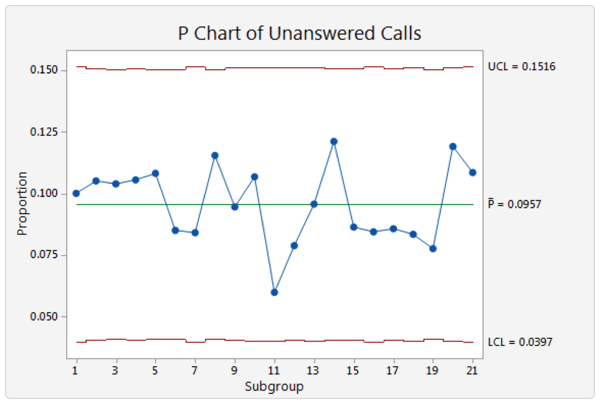
Can we really assume that the probability of each individual call going unanswered is exactly the same? Queuing theory tells us NO.
Here is a PBC with that same data:
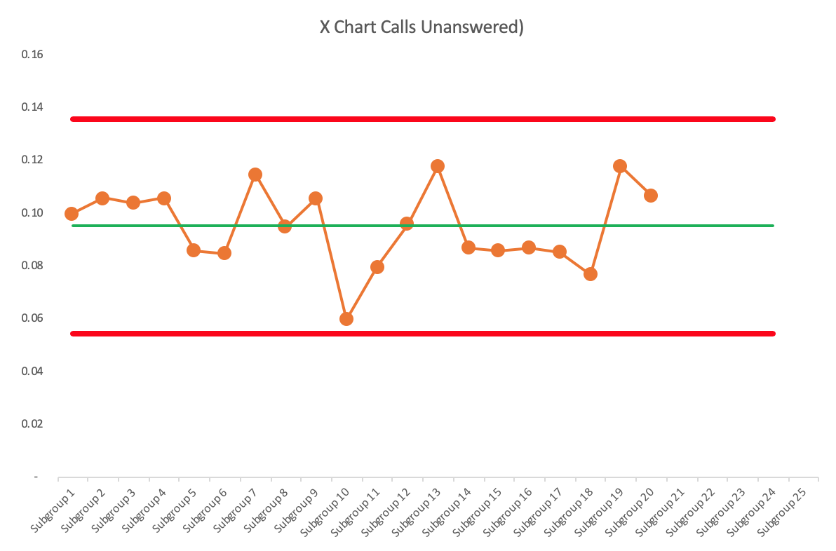
The PBC is easier to calculate and gives basically the same answer… without the bad assumption.
The c-chart and u-chart make also bad assumptions about the uniformity of what’s being measured and u-charts have the same varying-limits confusion as is caused by the p-charts.
Wheeler calls the XmR chart the “Swiss Army knife of control charts.” This website has a graphical flow chart for choosing the control type chart to use — it’s based on a diagram from Wheeler’s book.
When I have taught my workshop, I had one session where a Six Sigma Master Black Belt talk to me afterward and he said, basically, “My executives get lost and their eyes glaze over when I try explaining the various types of control charts. It’s great to have a single method that does the job well enough in all circumstances.”
What matters more is the thinking around our Process Behavior Charts. Can we stop from reacting to every up and down in a chart? Can we learn to filter out noise so we can find possible signals?
Wheeler also adds:
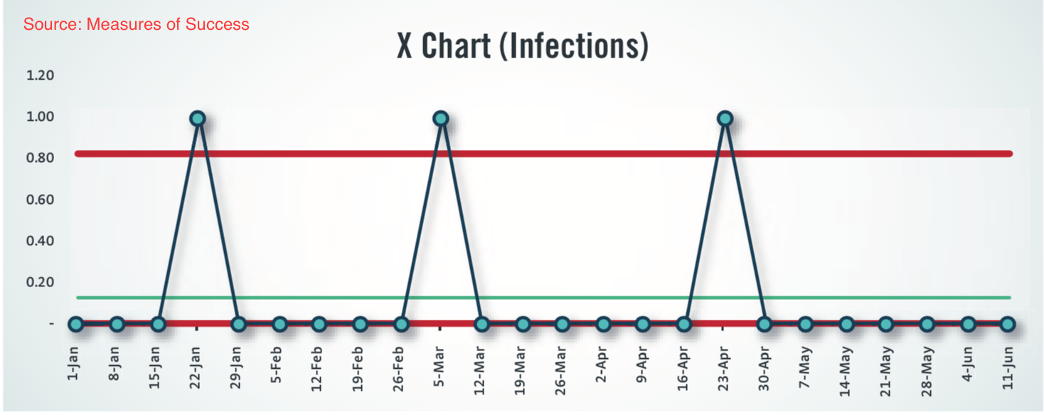
“The only instance of count data which cannot be reasonably placed on an XmR chart is that of very rare items or very rare events: data for which the average count per sample falls below 1.0.”
Wheeler addresses how to address this “chunky” data in his book.
For my readers, I address this in my book by offering a method of counting, for example, the days between rare events, like employee injuries or patient falls.
Below is the chart with an average <1:
And here is a chart of the days between infections:
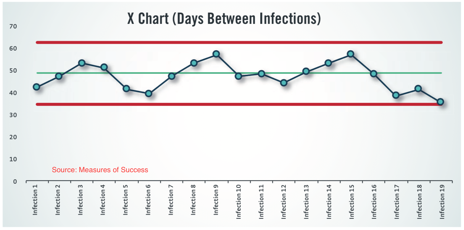
That addresses the “rare events” situation for many, if not all, cases.
Comments